Linear model
What is Linear model?
A linear model make a prediction by simply computing a weighted sum of the input features, plus a constant called the bias term (also called the intercept term).
\[\hat y = \theta_0 + \theta_1 x_1 + \cdots + \theta_n x_n\]Dataset
# generate linear-looking data plus some noise:
import numpy as np
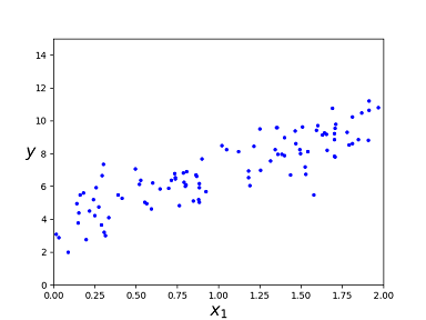
X = 2 * np.random.rand(100,1)
y = 4 + 3 * X + np.random.randn(100,1)
Plot the dataset in the following picture.
LinearRegression class
Perform Linear Regression using scikit-learn’s LinearRegression class.
from sklearn.linear_model import LinearRegression

lin_reg = LinearRegression()
lin_reg.fit(X, y)
lin_reg.intercept_, lin_reg.coef_
Out[3]: (array([4.32075143]), array([[2.80811042]]))

# the test set
X_new = np.array([[0],[2]])
y_lin_predict = lin_reg.predict(X_new)
y_lin_predict
Out[4]:
array([[4.32075143],
       [9.93697226]])
SGDRegressor class
Perform Linear Regression using scikit-learn’s SGDRegressor class.
from sklearn.linear_model import SGDRegressor

sgd_reg = SGDRegressor(max_iter=1000, tol=1e-3, penalty=None, eta0=0.1, random_state=42)
sgd_reg.fit(X, y.ravel())
Out[9]: SGDRegressor(eta0=0.1, penalty=None, random_state=42)

sgd_reg.intercept_, sgd_reg.coef_
Out[14]: (array([4.3270307]), array([2.87206748]))

y_sgd_predict = sgd_reg.predict(X_new)
y_sgd_predict
Out[16]: array([ 4.3270307 , 10.07116566])
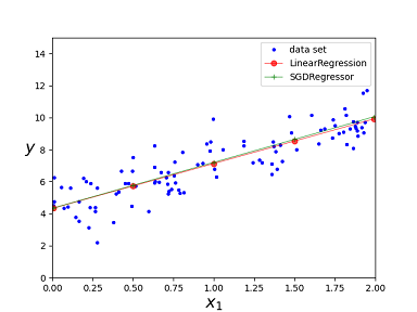
Plot the predictions from different algorithms
import matplotlib.pyplot as plt

# plot data set
plt.plot(X, y, "b.", label="data set")
plt.xlabel("$x_1$", fontsize=18)
plt.ylabel("$y$", rotation=0, fontsize=18)
plt.axis([0, 2, 0, 15])

X_test = np.array([[0.01], [0.5], [1], [1.5], [1.99]])
y_lin_predict = lin_reg.predict(X_test)
plt.plot(X_test, y_lin_predict, 'or-', lw=0.8, alpha=0.7, label='LinearRegression')

y_sgd_predict = sgd_reg.predict(X_test)
plt.plot(X_test, y_sgd_predict, "+g-", lw=0.8, alpha=0.7, label="SGDRegressor")
plt.legend()
Here is the plotting image:
Algorithms
The learning algorithms are discussed in Training a model. The scikit-learn doc gives more algorithms for the linear model.
If we look deeply at the previous algorithms and we’ll find that they may not work well on some cases.
The coefficient estimates for Ordinary Least Squares rely on the independence of the features. When features are correlated and the columns of the design matrix X have an approximate linear dependence, the design matrix becomes close to singular and as a result, the least-squares estimate becomes highly sensitive to random errors in the observed target, producing a large variance. This situation of multicollinearity can arise, for example, when data are collected without an experimental design.
SVD solution’s perspective
The SVD solution gives the model params:
\[\theta = \sum_{i=1}^r \frac{1}{\sigma_i}u_i^Tyv_i\]If the sigular value \(\sigma_i\) is very small, then the model params will be very large. Any noise in the observed target will be enlarged. Thus it lead to large variance of the model params.
Condition number’s perspective
One shall think of the condition number as being (very roughly) the rate at which the solution will change with respect to a change in the observed target.
The wikipedia condition number gives more detail of it. For a linear equation Ax = b, let e be the error in b. Assuming that A is a nonsingular matrix, the error in the solution \(A^{−1}b\) is \(A^{−1}e\). The ratio of the relative error in the solution to the relative error in b is
\[{\frac {\|A^{-1}e\|}{\|A^{-1}b\|}}/{\frac {\|e\|}{\|b\|}} = {\frac {\|A^{-1}e\|}{\|e\|}}{\frac {\|b\|}{\|A^{-1}b\|}} \leq \|A^{-1}\|\,\|A\| = \kappa (A)\]If \(\|\cdot \|\) is the norm defined in the square-summable sequence space, then
\[\kappa (A)={\frac {\sigma_{\text{max}}(A)}{\sigma_{\text{min}}(A)}}\]where \(\sigma_{\text{max}}(A)\) and \(\sigma_{\text{min}}(A)\) are maximal and minimal singular values of A respectively.
As we can see, small minimal singular value leads to big condition number, which means a big variance of the model params.
How to resolve this issue? We can take the Ridge Regression into consideration.