Data Collection and Visualization

There’re many tools for data collection and visualization. We shall be familiar with some of these tools.

As stated in its website, pandas is a fast, powerful, flexible and easy to use open source data analysis and manipulation tool, built on top of the Python programming language. We’ll use it for our investigation.

Suppose we want to find the relationship between happeness and wealth, we download the Better Life Index data from OECD’s website and GDP per capita data from the IMF’s website. Then we get two csv files: oecd_bli_2015.csv and gdp_per_capita.csv.

Merge data from these two files and then visualize it to get insights.

import os
import pandas as pd

datapath = os.path.join("datasets", "lifesat", "")

oecd_bli = pd.read_csv(datapath + "oecd_bli_2015.csv", thousands=',')
oecd_bli = oecd_bli[oecd_bli["INEQUALITY"]=="TOT"]
oecd_bli = oecd_bli.pivot(index="Country", columns="Indicator", values="Value")

gdp_per_capita = pd.read_csv(datapath+"gdp_per_capita.csv", thousands=',', delimiter='\t',
                             encoding='latin1', na_values="n/a")
gdp_per_capita.rename(columns={"2015": "GDP per capita"}, inplace=True)
gdp_per_capita.set_index("Country", inplace=True)

full_country_stats = pd.merge(left=oecd_bli, right=gdp_per_capita, left_index=True, right_index=True)
full_country_stats.sort_values(by="GDP per capita", inplace=True)

Get a table like following:

gdp_and_bli = full_country_stats[["GDP per capita","Life satisfaction"]]
gdp_and_bli.loc[["Hungary","Korea","France","Australia","United States"]].head()

Out[1]:
               GDP per capita  Life satisfaction
Country
Hungary             12239.894                4.9
Korea               27195.197                5.8
France              37675.006                6.5
Australia           50961.865                7.3
United States       55805.204                7.2

Visualize the data by pandas and matplotlib:

import matplotlib.pyplot as plt

gdp_and_bli.plot(kind='scatter', x="GDP per capita", y='Life satisfaction')
plt.axis([0, 60000, 0, 10])

gdp and better life index

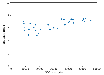
From the plot picture, we can assume there’s a “linear” relationship. And we can train it with a linear model.