02 Underlying Principles
Model of the cost function
As was discussed before, a neurone model contains params to be learnt from examples. We can develop a math model for investigation – a cost function:
\[\begin{equation*} C(w,b) = \frac{1}{2n} \sum_x \| y(x) - \hat{y}\|^2 \tag{2-1}\end{equation*}\]Our goal is to get the smallest C(w,b) which depends on value of w and b.
In other words, our goal is to get appropriate w and b that can
make a smallest C(w,b). How to get it?
Intuition of finding smallest cost
From the equation, we can take the cost function as a curved surface. Then go step by step from the initial point to the point whose cost function is smallest: \((w_0, b_0) \rightarrow \cdots \rightarrow (w_m, b_m), \; C_{min} = C(w_m, b_m)\)
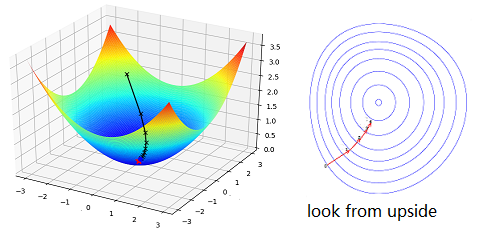
An efficient way is to walk with a proper step size towards the direction that goes down most quickly. We give the “step size” a name learning rate \(\eta\) and the direction a name gradient descent. \(\eta\) is to be adjusted by experience and “gradient descent” is a math concept. For the word “proper”, I mean that we can choose a proper \(\eta\) so that the point can walk with a big step size.
Get the step equation
The readers shall have basic foundation on Total devirative and Gradient. We’ll show how to get a “step” of a point, so that the cost function becomes smaller.
\(\begin{equation*} \Delta C \approx \frac{\partial C}{\partial w} \Delta w + \frac{\partial C}{\partial b} \Delta b \tag{2-2} \end{equation*}\) \(\begin{equation*} \mbox{gradient: } \; \nabla C \equiv \left( \frac{\partial C}{\partial w}, \frac{\partial C}{\partial b} \right)^T \tag{2-3} \end{equation*}\) \(\begin{equation*} \Delta C = \nabla C \cdot \Delta v, \;\;\; v = (w, b) \tag{2-4}\label{eq:dotproduct} \end{equation*}\)
We can design a “step size” to make the point walk towards the lowest point quickly:
\(\begin{eqnarray} \Delta v = -\eta \nabla C , \; i.e., \; v \rightarrow v' = v-\eta \nabla C \tag{2-5}\end{eqnarray}\) \(\begin{eqnarray} \Delta C = - \eta \|\nabla C\|^2 < 0 \tag{2-6}\end{eqnarray}\)
With \(\eta\), the point walks with a proper step size; with \((-1)\nabla C\), it walks towards the fast direction. And the cost function becomes smaller after this step.
Do you know why \(\pm \nabla C\) is the fast direction to increase/decrease?
From \(\eqref{eq:dotproduct}\), we know \(\Delta C\) is equal to dot product of two vectors.
And it gets the max value when the two vectors are in the same direction.
(from Cauchy–Schwarz inequality,
\({\displaystyle |\langle \mathbf {u} ,\mathbf {v} \rangle |\leq \|\mathbf {u} \|\|\mathbf {v} \|}\),
the two sides are equal if and only if u and vare linearly dependent)
Before we get to the final equation, let’s go back to defination of cost function (2-1). The cost function is an average of values that “cost” on every example: \(C = \frac{1}{n} \sum_x C_x\). Thus we have \(\nabla C = \frac{1}{n} \sum_x \nabla C_x\). Now we have the step equation:
\[\begin{eqnarray} w_k & \rightarrow & w_k' = w_k-\frac{\eta}{n} \sum_j \frac{\partial C_{X_j}}{\partial w_k} \\ b_l & \rightarrow & b_l' = b_l-\frac{\eta}{n} \sum_j \frac{\partial C_{X_j}}{\partial b_l} \tag{2-7}\label{eq:step}\end{eqnarray}\]Algrithm
Now we come to the final algrithm:
- take intial values: \(w_0, \; b_0\)
- with the step equation \(\eqref{eq:step}\), walks one step each time to get a smaller cost function
- repeat the process until the cost is small enough